This first tutorial will guide you through testing the correct installation of cLASpy_T. The tutorial assumes that the installation is clomplete and that the venv is operational. If this is not the case, see Install.
Explore Dataset
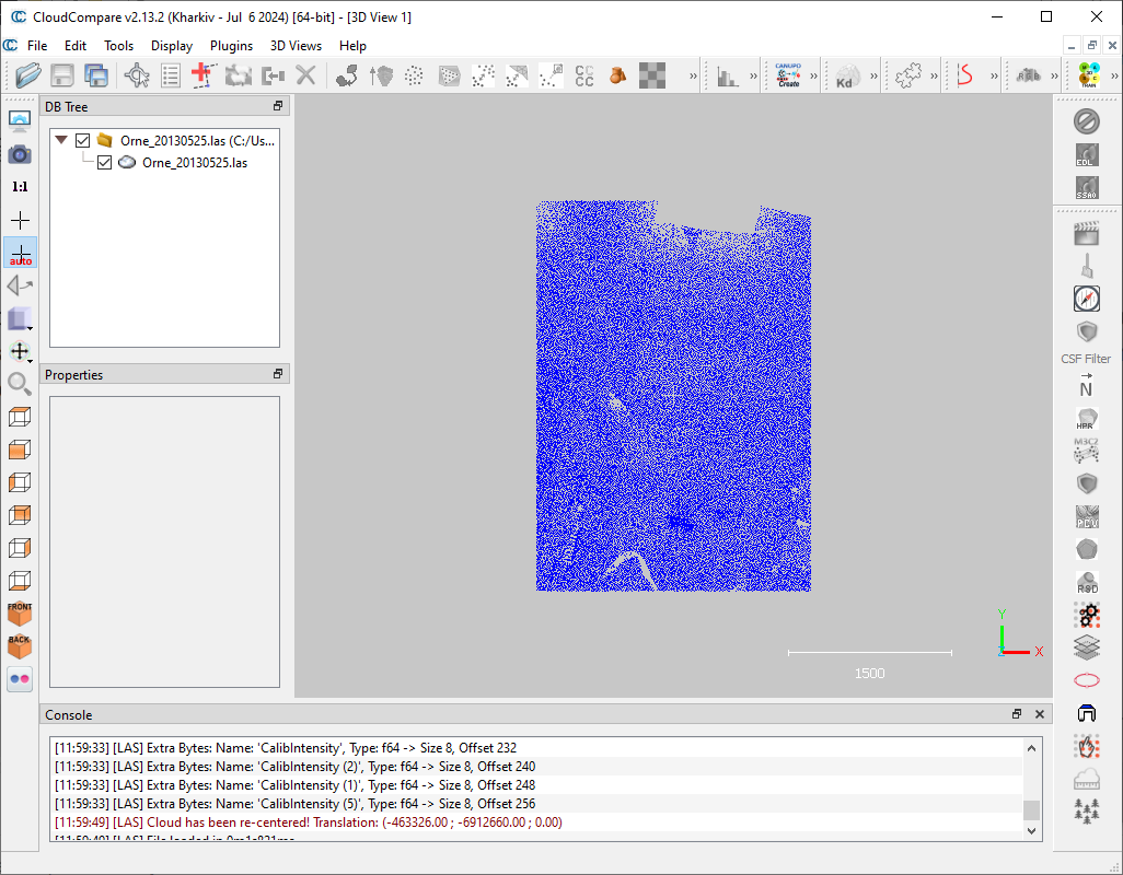
Using point cloud visualization software such as CloudCompare, open the Test/Orne_20130525.las file in the cLASpy_T root directory.
You should see something like this:
Note
This point cloud is too light (only 50,000 points) to correspond to a real use case, but it’s useful to test that cLASpy_T works.
To create an automatic classification model, different types of data are required. These are labels, which identify the class to which each point belongs, and features, which describe each point.
Labels
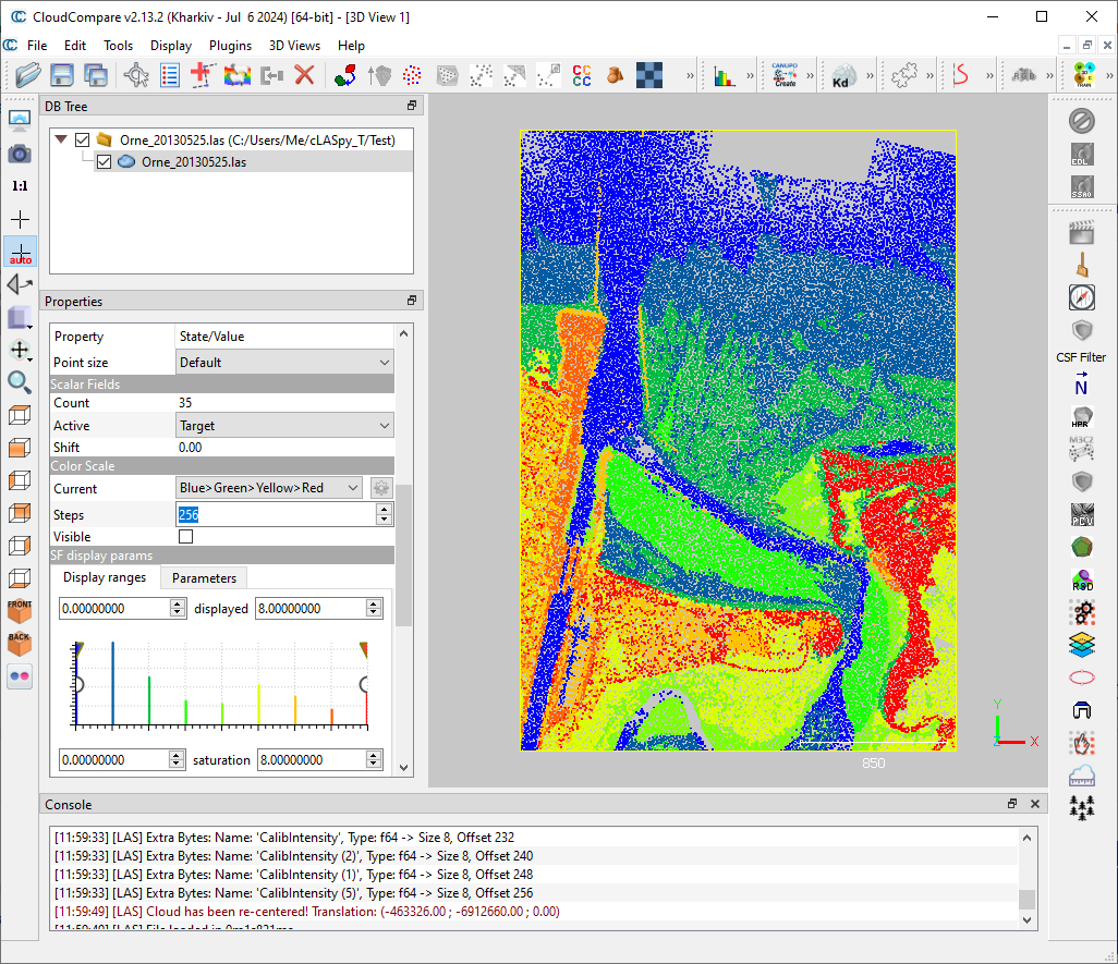
Labels are contained in the ‘Target’ scalar field.
You can view these labels by selecting the point cloud Orne_20130525.las, then in Scalar Fields, scroll down and select ‘Target’.
You see 9 classes, from 0 to 8 as follow:
Water
Wet sand
Dry sand
Mix (sand + mud)
Mud
Grass and Schorre
High vegetation and Buildings
Roads
Low vegetation
Features
Features are all other scalar fields such as ‘Roughness (5)’, ‘Omnivariance (10)’, ‘R’, ‘G’, ‘B’ or ‘Return Number’.
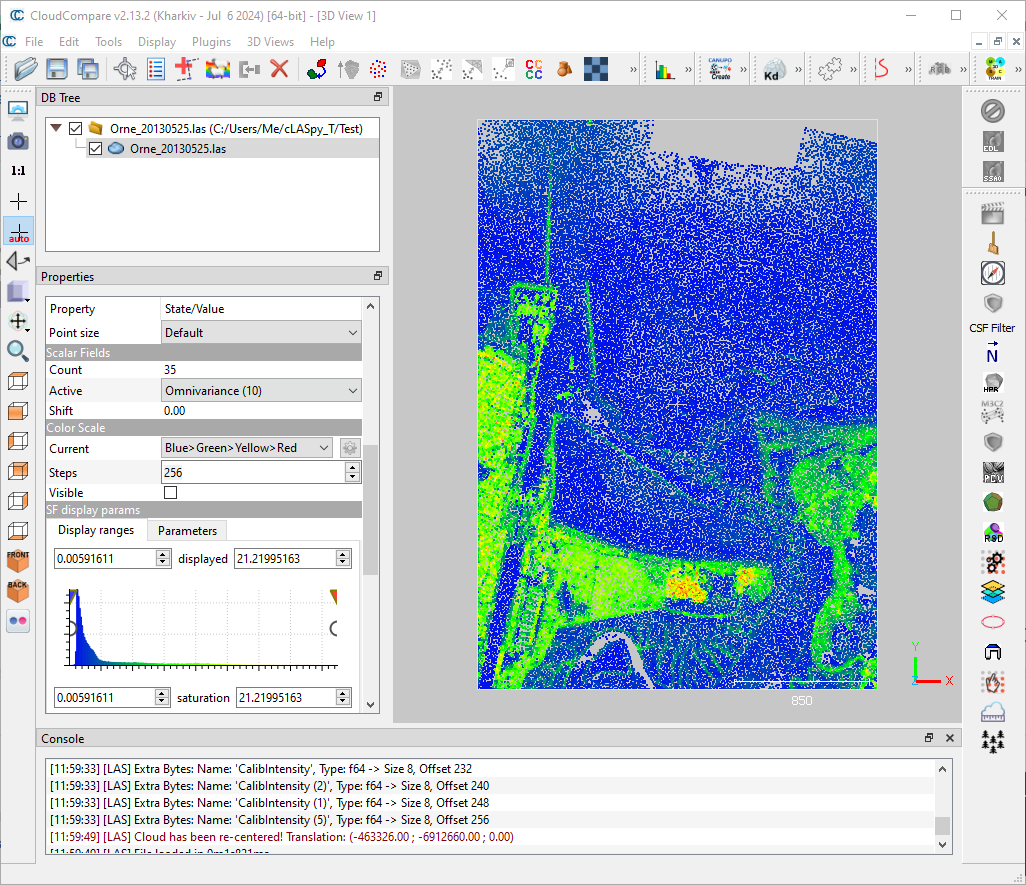
The goal of a supervised machine learning algorithms is to model the membership of points to their class, or their label/target, based on input features. The choice of these features is therefore essential for a consistent and robust model.
Test command-line
The first step is to test cLASpy_T command line, to ensure all library dependencies are properly installed.
You will create a classification model by running a training session with the ‘train’ module and the very light point cloud Orne_20130525.las in the Test folder of the cLASpy_T sources.
This point cloud contains the ‘Target’ scalar field and the features needed for training.
Then, you will use the model you created to make predictions on the same point cloud, to ensure that the ‘predict’ module is also fully operational.
If all goes well, you should obtain a folder containing 4 files: a model, a LAS point cloud and two reports, one for training and the other for prediction.
First run
Activate the Python virtual environment (venv) created during installation process, from the cLASpy_T folder.
On Windows:
C:\Users\Me\Code\cLASpy_T>.venv\claspy_venv\Scripts\activate
On Linux:
me@pc:~/Code/cLASpy_T$ source .venv/claspy_venv/bin/activate
cLASpy_T consists of 3 modules: ‘train’, ‘predict’ and ‘segment’. The first and second are used to train a supervised model and make predictions. The ‘segment’ module perform unsupervised machine learning, with the KMeans algorithm.
You can get more details about cLASpy_T and modules with --help command.
Example: help for ‘predict’ module
python cLASpy_T.py predict --help
usage: cLASpy_T.py predict [-h] [-c] [-i] [-o] [-m] [--fillnan]

-------------------------------------------------------------------------------

                          cLASpy_T
                      predict sub-command
                  =========================

'predict' makes predictions on the input point cloud according the selected model.

For predictions, two files are required:
  --> the input_data file with the same features used to create the model.
  --> the '*.model' file created during the training phase.

-------------------------------------------------------------------------------

options:
  -h, --help          show this help message and exit
  -c , --config       give the configuration file with all parameters
                          and selected scalar fields.
                          [WINDOWS]: 'X:/path/to/the/config.json'
                          [UNIX]: '/path/to/the/config.json'

  -i , --input_data   set the input data file:
                          [WINDOWS]: 'X:/path/to/the/input_data.file'
                          [UNIX]: '/path/to/the/input_data.file'

  -o , --output       set the output folder to save all result files:
                          [WINDOWS]: 'X:/path/to/the/output/folder'
                          [UNIX]: '/path/to/the/output/folder'
                          Default: '/path/to/the/input_data/'

  -m , --model        import the model file to make predictions:
                          '/path/to/the/training/file.model'

  --fillnan           set the value to fill NaN for feature values.
                          Could be 'median', 'mean', int or float.
                          Default: '--fillnan='median'
Note
If it doesn’t work, check the cLASpy_T dependencies are installed, as explained in the Install section.
Training
To train your first model with the ‘train’ module, you need to set the algorithm and the input file. All other arguments of ‘train’ module are optional.
Run the following command to train a basic RandomForestClassifier model.
python cLASpy_T.py train -a=rf -i=./Test/Orne_20130525.las
-a: set the supervised algorithm, here rf refers to RandomForestClassifier
-i: set the point cloud file, here
Orne_20130525.las
Training Ouput
The first part of the terminal output shows the cLASpy_T mode, the algorithm used and the input data file.
# # # # # # # # # #  cLASpy_T  # # # # # # # # # # # #
- - - - - - - -    TRAIN MODE    - - - - - - - - - -
* * * *    Point Cloud Classification    * * * * * *

Algorithm used: RandomForestClassifier
Path to LAS file: Test\Orne_20130525.las

Create a new folder to store the result files... Done.
Once the file has been loaded, the output shows the LAS format and the total number of points. Then, the cLASpy_T pipeline starts, with the input data formatted in pandas.DataFrame (see 10 minutes to pandas).
If no list of selected features is provided with --features (-f) argument, the default behavior of cLASpy_T is to retrieve all extra dimensions from the LAS file as selected features. The standard LAS file dimensions are discarded by default.
The ‘train’ module also search the ‘Target’ field in the data and shows the labels used. Here, there are 9 labels, from 0 to 8 as already seen with CloudCompare.
LAS Version: 1.2
LAS point format: 1
Number of points: 50,000

Step 1/7: Formatting data as pandas.DataFrame...

All features in input_data will be used!
Except X, Y, Z and LAS standard dimensions!

LABELS FROM DATASET:
[0, 1, 2, 3, 4, 5, 6, 7, 8]
The second step of the cLASpy_T pipeline is to split dataset into train and test sets, according to the --train_r: the training ratio. Here, the train and test sets are 25,000 points each, according the default --train_r =0.5.
The third step scales the dataset according the --scaler selected: StandardScaler, MinMaxScaler or RobustScaler (see scalers).
Step 2/7: Splitting data in train and test sets...

Random state to split data: 0
        Number of used points: 50 000 pts
        Size of train|test datasets: 25 000 pts | 25 000 pts

Step 3/7: Scaling data...
Warning
With large dataset, this step consumes a lot of RAM and can take a long time if memory is full. If cLASpy_T stops at this stage with RAM full, reduce the size of the point cloud, or increase the computer’s RAM capacity.
Step 4/7 is the actual model training. Depending on the point cloud size, the algorithm used and the number of features and classes, this step is often the longest. It can last from a few minutes to several hours.
The training uses the cross-validation method (CV for short) to ensure robust models. So, 5 training are performed simultaneously on 5 subsets of trainset (see cross-validation). Here, the training set is composed of 25,000 points, so 5 subsets of 5,000 points are created. Each subset, or fold, is used once to test the model trained with the other 4 folds.
Once done, cLASpy_T returns the global accuracy of the 5 sub-models. To check that the model is consistent and robust, the 5 scores must be close to each other. If one or more scores are several units (%) apart, there is a problem with the classes, features, model or training parameters.
Step 4/7: Training model with cross validation...

Random state for the StratifiedShuffleSplit: 0

        Training model scores with cross-validation:
        [0.6934 0.6918 0.6898 0.6878 0.6862]

Model trained!
Note
Check CPUs are working to make sure that cLASpy_T isn’t freezing. The number of CPUs used by cLASpy_T can be set with --n_jobs argument.
After training, cLASpy_T tests the model by making predictions on the 25,000 points of the test set, created during step 2/7. The results are presented in the form of a confusion matrix and a classification report.
The confusion matrix allows to explore in detail the predictions made by the model for each point. The columns present the predictions made by the model, while the rows correspond to the expected classes for each point. The end of each column corresponds to the precision of each class, while the end of each row corresponds to the recall of each class. The global accuracy is the end of the last line, here: 69.6%.
The classification report exposes the same results by classes, with the number of points for each class (support).
Step 5/7: Creating confusion matrix...

CONFUSION MATRIX:
Predicted         0         1        2        3        4         5         6        7         8  Recall
True
0          5064.000   194.000     1.00   16.000    3.000   126.000    21.000   32.000    10.000   0.926
1           355.000  4635.000   367.00   34.000   27.000    29.000     3.000    7.000     2.000   0.849
2             1.000   769.000  2347.00    4.000    0.000    19.000     1.000    7.000    24.000   0.740
3           364.000   735.000    65.00  248.000   15.000   169.000     0.000   10.000     6.000   0.154
4           115.000   794.000    16.00   92.000  151.000    89.000    44.000   75.000    40.000   0.107
5           128.000    40.000    14.00   17.000    6.000  1808.000   200.000   14.000   417.000   0.684
6            20.000     5.000    11.00    1.000    4.000    60.000  1324.000   35.000   419.000   0.705
7           377.000    31.000    23.00    5.000   28.000    60.000   223.000  185.000   104.000   0.179
8             2.000    17.000    53.00    2.000    1.000   168.000   420.000   16.000  1636.000   0.707
Precision     0.788     0.642     0.81    0.592    0.643     0.715     0.592    0.486     0.616   0.696

TEST REPORT:
              precision    recall  f1-score   support

          0       0.79      0.93      0.85      5467
          1       0.64      0.85      0.73      5459
          2       0.81      0.74      0.77      3172
          3       0.59      0.15      0.24      1612
          4       0.64      0.11      0.18      1416
          5       0.72      0.68      0.70      2644
          6       0.59      0.70      0.64      1879
          7       0.49      0.18      0.26      1036
          8       0.62      0.71      0.66      2315

    accuracy                           0.70     25000
  macro avg       0.65      0.56      0.56     25000
weighted avg       0.69      0.70      0.66     25000
The step 6/7 save the model, and all other needed parameters such as scaler, in a binary file with a .model extension.
This binary file is created with joblib python library.
The last step writes all relevant training parameters to a report file.
Step 6/7: Saving model and scaler in file:

Model path: Test\Orne_20130525/
Model file: train_rf50kpts_1217_1619.model

Step 7/7: Creating classification report:
Test\Orne_20130525/train_rf50kpts_1217_1619.txt

Training done in 0:00:03.095406
Note
Bravo ! You trained your first machine learning model with cLASpy_T.
Prediction
You now have a trained machine learning model. We’ll use it on the same dataset with the ‘predict’ module to make predictions and check that this module is working properly.
To use your first model with the ‘predict’ module, you must pass the .model file with the -m argument and set the input file.
All other arguments of ‘predict’ module are optional.
Run the following command to make prediction with your model.
python cLASpy_T.py predict -m=Test/Orne_20130525/train_gb50kpts_mmjj_HHMM.model -i=Test/Orne_20130525.las
-m: set the model to make predictions, change
train_gb50kpts_mmjj_HHMM.modelwith your model file.-i: set the point cloud file, here
Orne_20130525.las
Prediction Ouput
The first part of the terminal output shows the cLASpy_T mode.
At the first step, cLASpy_T loads the model and gives the labels, the original algorithm and the input data file. Once the file has been loaded, the output shows the LAS format and the total number of points.
# # # # # # # # # #  cLASpy_T  # # # # # # # # # # # #
- - - - - - - -    PREDICT MODE    - - - - - - - - - -
* * * * *    Point Cloud Classification    * * * * * *

Step 1/6: Loading model...
LABELS FROM MODEL:
[0, 1, 2, 3, 4, 5, 6, 7, 8]

      Any PCA data to load from model.

Algorithm used: RandomForestClassifier
Path to LAS file: Test\Orne_20130525.las

Create a new folder to store the result files... Folder already exists.

LAS Version: 1.2
LAS point format: 1
Number of points: 50,000
The second step, the ‘predict’ module format data as pandas.DataFrame and check that all features used by the model are in the input data. At this point, the ‘Target’ field is discarded if present.
Step 2/6: Formatting data as pandas.DataFrame...

Get selected features:
- roughness_(2) asked --> Roughness (2) found
- surface_variation_(10) asked --> Surface variation (10) found
- eigenentropy_(10) asked --> Eigenentropy (10) found
- anisotropy_(2) asked --> Anisotropy (2) found
- g asked --> G found
...
...
...
- omnivariance_(5) asked --> Omnivariance (5) found
- saturation asked --> Saturation found
- anisotropy_(10) asked --> Anisotropy (10) found
- omnivariance_(2) asked --> Omnivariance (2) found
- calibintensity_(5) asked --> CalibIntensity (5) found
- original_intensity asked --> Original_Intensity found
- sphericity_(10) asked --> Sphericity (10) found
- surface_variation_(5) asked --> Surface variation (5) found

Number of selected features: 32
Number of final used features: 32
--> All required features are present!